How to Collect and Log Web Clickstream Data

Clickstream Data

What is clickstream data?

The path a user takes through a website is generally referred to as the user's clickstream.

Why collect clickstream data?

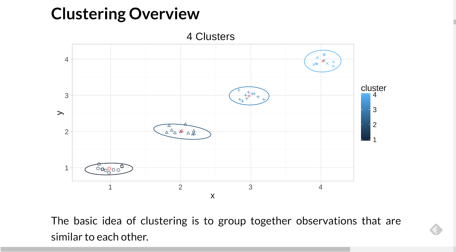
When aggregated using map-reduce techniques and then using unsupervised machine learning predictive analytics techniques like clustering and association analysis, clickstream data can tell you many things, including

• how users use your site
• if there are different behavioral groups within users
• what marketing works or does not work

Clickstream data can also be used to build recommender systems, perform ROI analysis on marketing (via Shapley values), and improve lead scoring

Client-side collection

Since a lot of the traffic to most websites is bot traffic, it is helpful to collect via client-side script as many bots do not evaluate JavaScript and many legitimate bots (e.g. search-engine spiders) identify themselves as such.

A simple method for collection is to add a <script> tag with an immediately-invoked function expression (IIFE) just before the closing </body> tag. An example of such a script is shown below.

The code above simply creates an image tag in code and assigns a source to it. The assignment of a src value causes the browser to fetch the requested resource.

• Cache busting
  Since many browsers cache static resources, a random value is added to the URL as a cache buster.
• Referrer
  For the purposes of clickstream data, it is useful to include the URL of the page that caused the current page to be loaded; this is called the "referrer" and is added to the pixel image URL as a parameter named "dr" (the name is "dr" is used to conform to the parameter names used in the Google Analytics Measurement Protocol.

Server-side ASP.NET MVC Listener

Pixel Endpoint

The code on the server side has three primary responsibilities:

1. to set/update certain cookie values (explained below),
2. to log the values, and
3. to return something that the browser will accept (this response will carry the cookies)

Cookies

In general, there are four anonymous values that need to be tracked (if your site allows users to log in, it may be useful to add a fifth cookie to allow you to aggregate cross-device behavior). The values to be tracked/collected are:

• Session ID
  A temporary anonymous identifier that allows you to group together the page view records captured by the end point. The value will be different each time the user visits your site anew but will remain constant while the user is using your site.
• Sequence #
  A temporary integer value that allows you to order the page view log records. The value will increment as the user navigates the site.
• Client ID
  A semi-permanent anonymous identifier that allows you to group together multiple sessions from the same browser/client. NOTE: the value is specific to the browser/machine/user combination: a different logged in user on a machine will have a different client ID; if the same user uses multiple browsers (e.g. Chrome and Firefox), each browser will have a unique client ID.
• Session count
  A semi-permanent anonymous identifier that allows you to analyze how user behavior changes over subsequent visits.

Getting the value of a cookie from the client request

The code for retrieving a cookie value from the client request is fairly straight-forward. One needs to guard against the case where the cookie does not exist.

Incrementing the sequence value

The "seq" cookie is simply a counter. It, along with the time of the request, which is logged, allows the analyst to study how users navigate a site. Along with the previous page, which is passed up as the "dr" parameter, the sequence value is useful for multi-tab browsing scenarios.

Incrementing the session count

A new session will not have a session ID. If this is the case, the session count needs to be incremented. The session count cookie should be semi-permanent.

Setting the client ID

The client ID should be semi-permanent and should only be set if there is not one already set.

Setting the session ID

The session ID is a temporary value. It's value will be cleared when the user closes the browser. Although it may be tempting to define a session timeout period, since any value chosen will be arbitrary, it is important that the data logged be agnostic and that any session timeout adjustments desired be done during analysis.

Setting cookie values

To safeguard the cookie values and the user, it is important that the cookies be set to be HTTP-only (preventing client script and browser plugin/addon tampering), that the cookies be secure (i.e. HTTPS-only – your site should be HTTPS-only).

To make your pixel useful over all of your web assets, it is helpful to set the domain. Suppose you have domain names like the following:

• www.example.com
• blog.example.com
• response.example.com

To have one pixel connect your users over all of these domains, simply set the domain of the cookie to "example.com".

Logging Values

Given the power of Map-Reduce technologies that are available in Hadoop, R, MongoDB, etc., it makes sense to store the initial data in JSON format.

Four additional pieces of information are added to the serialized data.

• the time,
• the user agent
  which is useful for distinguishing mobile from desktop sessions,
• the page calling the pixel end point, and
• the referring page that caused the page with the pixel code to be loaded

The code for serializing the values follows:

Full code with unit tests

The full source code for this article is available at https://github.com/stand-sure/Clickstream

Predicting 2016 Presidential Election Results via Clustering

Goal

The goal of this article is to

• Predict how undecided states will vote in the 2016 Presidential Election

using

• U.S. Presidential Election results from 1980 - 2012
• data indicating which states that are likely to vote for either Mrs. Clinton or Mr. Trump in 2016

The states that are omitted are the undecided states for which predictions are made.

Business Applications

Suppose

• candidates = products
• states = consumers

Then the following things can be inferred using the method shown in this article:

• Consumer Characteristics:
• Birds of a feather flock together.
• If data from a new consumer is collected,
• the new consumer probably shares qualitative/meta traits with the group to which (s)he appears to belong.
• Different marketing messages might make sense based on the inferred demographic and psychographic traits.
• Lead scoring:
• It is likely that new consumers will behave in the same way in the sales process as other members of their group have performed.
• If the number of prospects exceeds the capacity of sales professionals, prioritizing the prospects in clusters that have historically performed better should improve business results.
• Preference prediction/Recommender systems:
• It is likely that if a consumer “likes” a product, (s)he will probably also like another product in the product’s cluster. (“Like” can mean a product view, shopping cart action, purchase, etc.)
• A “similar products” section (with more domain-specific wording) on the product page(s) on your website may cause users to look at more products (increasing time on site, pages/session and (hopefully) leads and sales).
• Marketing emails recommending these products may also be useful.

Clustering Overview

The basic idea of clustering is to group together observations that are similar to each other.

Visually, our brains understand clustering. In the image above, there appear to be four groupings in the data.

When there are more than two variables being observed, an algorithmic approach is useful.

Election Data

The raw election data used in this article is in the form:

 state candidate year votes party
1    AK     Obama 2012     0     D
2    AL     Obama 2012     0     D
3    AR     Obama 2012     0     D
4    AZ     Obama 2012     0     D
5    CA     Obama 2012    55     D
6    CO     Obama 2012     9     D

The data is transformed using functions found in the packages:

• plyr
• dplyr
• tidyr

To make the code more readable, the pipe operators from the package magrittr are used.

Below is an example of data manipulation.

candidateParty <- results %>%
 select(year, candidate, party) %>%
 distinct() %>%
 arrange(year, candidate, party)

There is a row for each candidate who received electoral college votes for each state in each election year.

Vote Totals

EC Votes by Year and candidate

year	candidate	votes	year	candidate	votes
1980	Carter	49	1996	Dole	159
1980	Reagan	490	2000	Bush	271
1984	Mondale	13	2000	Gore	266
1984	Reagan	524	2004	Bush	286
1988	Bentsen	1	2004	Kerry	251
1988	Bush	426	2008	McCain	173
1988	Dukakis	111	2008	Obama	365
1992	Bush	168	2012	Obama	332
1992	Clinton	370	2012	Romney	206
1996	Clinton	379	NA	NA	NA

Summary Results

Winner by Year

year	candidate	party
1980	Reagan	R
1984	Reagan	R
1988	Bush	R
1992	Clinton	D
1996	Clinton	D
2000	Bush	R
2004	Bush	R
2008	Obama	D
2012	Obama	D

% of time state predicts winner

State	Win Rate	State	Win Rate	State	Win Rate
AK	0.556	KY	0.778	NY	0.667
AL	0.556	LA	0.778	OH	1.000
AR	0.778	MA	0.667	OK	0.556
AZ	0.667	MD	0.667	OR	0.667
CA	0.778	ME	0.778	PA	0.778
CO	0.889	MI	0.778	RI	0.556
CT	0.778	MN	0.444	SC	0.556
DC	0.444	MO	0.778	SD	0.556
DE	0.778	MS	0.556	TN	0.778
FL	0.889	MT	0.667	TX	0.556
GA	0.556	NC	0.667	UT	0.556
HI	0.556	ND	0.556	VA	0.778
IA	0.778	NE	0.600	VT	0.778
ID	0.556	NH	0.889	WA	0.667
IL	0.778	NJ	0.778	WI	0.667
IN	0.667	NM	0.889	WV	0.556
KS	0.556	NV	1.000	WY	0.556

State party rates

State	Dem	Rep	State	Dem	Rep	State	Dem	Rep
AK	0.00	1.00	KY	0.22	0.78	NY	0.78	0.22
AL	0.00	1.00	LA	0.22	0.78	OH	0.44	0.56
AR	0.22	0.78	MA	0.78	0.22	OK	0.00	1.00
AZ	0.11	0.89	MD	0.78	0.22	OR	0.78	0.22
CA	0.67	0.33	ME	0.67	0.33	PA	0.67	0.33
CO	0.33	0.67	MI	0.67	0.33	RI	0.89	0.11
CT	0.67	0.33	MN	1.00	0.00	SC	0.00	1.00
DC	1.00	0.00	MO	0.22	0.78	SD	0.00	1.00
DE	0.67	0.33	MS	0.00	1.00	TN	0.22	0.78
FL	0.33	0.67	MT	0.11	0.89	TX	0.00	1.00
GA	0.22	0.78	NC	0.11	0.89	UT	0.00	1.00
HI	0.89	0.11	ND	0.00	1.00	VA	0.22	0.78
IA	0.67	0.33	NE	0.10	0.90	VT	0.67	0.33
ID	0.00	1.00	NH	0.56	0.44	WA	0.78	0.22
IL	0.67	0.33	NJ	0.67	0.33	WI	0.78	0.22
IN	0.11	0.89	NM	0.56	0.44	WV	0.44	0.56
KS	0.00	1.00	NV	0.44	0.56	WY	0.00	1.00

State Clusters

One question to figure out is how many clusters to use.

If one wants a numeric way to estimate the number of clusters to use the nScree function from the nFactors package, as follows:

states[,-1] %>%
 nFactors::nScree() %>%
 nFactors::plotnScree()

The suggested number of clusters is a good minimum to use.

Since it is important that cluster assignments have business/analytical value, it is generally useful to increase the number of clusters (provided they are stable) until useful distinctions based on other data stand out.

kmeans clustering

kmeans is an automated approach to clustering that works as follows:

1. k random centers are selected within the bounds of the data (you pick the value of k)
2. the distance between each data point and each random center is calculated and the data point is assigned to the cluster corresponding to the nearest center
3. the centers are then recalculated as the mean (a.k.a. average) of the points in the cluster
4. Steps #2 and #3 are repeated until the centers stop moving (or until the maximum number of iterations allowed is reached (this prevents infinite loops))

It should be noted that different runs of a kmeans algorithm can produce different clusters based on which random centers are used at the beginning of the algorithm. This is an effect of the algorithm and not the data.

In the snippet below, code is shown to calculate 6 clusters from the state data. The first column, which contains the state name, is excluded and only the 0/1 preference columns are used.

The code also shows an easy way to plot clusters, via clusplot from the cluster package [note: clusplot needs more (non-parallel) rows than columns].

set.seed(8675309)
nCenters <- 6
states.km <- states[,-1] %>%
 kmeans(centers = nCenters,
        nstart = 1e2)
clstr <- states.km$cluster

library(cluster)

clusplot2 <- Curry(clusplot,
                  color=T,
                  shade=T,
                  lines=0,
                  labels=2)

clusplot2(states[,-1],
         clstr,
         main = "States")

clusterboot

One of the key clustering challenges is determining if the cluster is “real”.

The centers initially chosen by the kmeans algorithm can impact the result.

One way to see if the clusters are “real” is to see if they hold up when variations of the data are used via a sampling process that allows replacement (this is called bootstrapping).

The clusterboot function in the fpc package performs bootstrap resampling and repeatedly runs the clustering algorithm indicated.

library(fpc)
nRuns = 100

clusterboot2 <- Curry(clusterboot,
                     clustermethod = kmeansCBI,
                     runs = nRuns,
                     iter.max = 1000,
                     seed = 8675309,
                     count = F)

suppressWarnings({
 states.cboot <- clusterboot2(states[,-1],
                              krange = nCenters)
})

clstr <- states.cboot$partition
clusplot2(states[,-1],
         clstr,
         main = "States")

stabilities <- states.cboot$bootmean %>%
 cut(breaks=c(0,
              0.6,
              0.75,
              0.85,
              1),
     labels=c("unstable",
              "measuring something",
              "stable",
              "highly stable"))

Cluster 1 - highly stable - breakdown rate: 0.03

state	demRate	repRate	winRate
CA	0.67	0.33	0.78
CT	0.67	0.33	0.78
DE	0.67	0.33	0.78
IL	0.67	0.33	0.78
MD	0.78	0.22	0.67
ME	0.67	0.33	0.78
MI	0.67	0.33	0.78
NH	0.56	0.44	0.89
NJ	0.67	0.33	0.78
NM	0.56	0.44	0.89
PA	0.67	0.33	0.78
VT	0.67	0.33	0.78

Cluster 1

Dem	Rep	Win
0.66	0.34	0.79

Cluster 2 - stable - breakdown rate: 0.26

state	demRate	repRate	winRate
DC	1.00	0.00	0.44
HI	0.89	0.11	0.56
MN	1.00	0.00	0.44
RI	0.89	0.11	0.56

Cluster 2

Dem	Rep	Win
0.94	0.06	0.5

Cluster 3 - stable - breakdown rate: 0.12

state	demRate	repRate	winRate
IA	0.67	0.33	0.78
MA	0.78	0.22	0.67
NY	0.78	0.22	0.67
OR	0.78	0.22	0.67
WA	0.78	0.22	0.67
WI	0.78	0.22	0.67

Cluster 3

Dem	Rep	Win
0.76	0.24	0.69

Cluster 4 - highly stable - breakdown rate: 0

state	demRate	repRate	winRate
AK	0.00	1.00	0.56
AL	0.00	1.00	0.56
AZ	0.11	0.89	0.67
ID	0.00	1.00	0.56
IN	0.11	0.89	0.67
KS	0.00	1.00	0.56
MS	0.00	1.00	0.56
NC	0.11	0.89	0.67
ND	0.00	1.00	0.56
NE	0.10	0.90	0.60
OK	0.00	1.00	0.56
SC	0.00	1.00	0.56
SD	0.00	1.00	0.56
TX	0.00	1.00	0.56
UT	0.00	1.00	0.56
WY	0.00	1.00	0.56

Cluster 4

Dem	Rep	Win
0.03	0.97	0.58

Cluster 5 - stable - breakdown rate: 0.07

state	demRate	repRate	winRate
AR	0.22	0.78	0.78
GA	0.22	0.78	0.56
KY	0.22	0.78	0.78
LA	0.22	0.78	0.78
MO	0.22	0.78	0.78
MT	0.11	0.89	0.67
TN	0.22	0.78	0.78
WV	0.44	0.56	0.56

Cluster 5

Dem	Rep	Win
0.24	0.76	0.71

Cluster 6 - highly stable - breakdown rate: 0.12

state	demRate	repRate	winRate
CO	0.33	0.67	0.89
FL	0.33	0.67	0.89
NV	0.44	0.56	1.00
OH	0.44	0.56	1.00
VA	0.22	0.78	0.78

Cluster 6

Dem	Rep	Win
0.36	0.64	0.91

Candidate Clusters

Below is the code to create candidate clusters. The first three columns contain non-preference data and are not used in the cluster computation.

Because there are fewer rows than columns, a cluster plot is not possible without some manipulation.

candidates <- results %>%
 spread(state, votes)

candidates[,-c(1:3)] <- ifelse(candidates[,-c(1:3)]>0,1,0)

nCenters <- 8
candidates %<>%
 as.data.frame()
rownames(candidates) <-
 paste(candidates$candidate, candidates$year)
suppressWarnings({
 candidates.cb <- clusterboot2(
   candidates[,-c(1:3)],
   krange = nCenters)
})

# hack to print a candidates graph
# clusplot(candidates[,-c(1:3)], candidates.cb$partition, ...) would fail
# because there are more columns (variables) than rows (observations)
# SVD is a technique used to factor the data into three matrices
# it discovers "latent" variables and concentrates the most significant to be first
# it is useful for reducing the number of dimensions to improve computational time
# the u matrix represents the rows rotated (candidates)
# the d matrix is a diagonal that represents scaling factors (i.e. strength)
# the v matrix represents the columns rotated (states)
# the hack here allows us to have two coordinates to plot
u <- candidates[,-c(1:3)] %>%
 svd() %$%
 u
rownames(u) <- paste(candidates$candidate, candidates$year)
clusplot2(u,
         candidates.cb$partition,
         main = "Candidates")

Cluster 1 - stable - breakdown rate: 0.23

Candidate	Year	Party	Outcome
Gore	2000	D	lose
Kerry	2004	D	lose

Cluster 2 - stable - breakdown rate: 0.21

Candidate	Year	Party	Outcome
Bush	2000	R	win
Bush	2004	R	win

Cluster 3 - highly stable - breakdown rate: 0.12

Candidate	Year	Party	Outcome
Bush	1992	R	lose
Dole	1996	R	lose

Cluster 4 - stable - breakdown rate: 0.31

Candidate	Year	Party	Outcome
Obama	2008	D	win
Obama	2012	D	win

Cluster 5 - stable - breakdown rate: 0.27

Candidate	Year	Party	Outcome
Bush	1988	R	win
Reagan	1980	R	win
Reagan	1984	R	win

Cluster 6 - stable - breakdown rate: 0.17

Candidate	Year	Party	Outcome
Bentsen	1988	D	lose
Carter	1980	D	lose
Dukakis	1988	D	lose
Mondale	1984	D	lose

Cluster 7 - highly stable - breakdown rate: 0.1

Candidate	Year	Party	Outcome
Clinton	1992	D	win
Clinton	1996	D	win

Cluster 8 - stable - breakdown rate: 0.22

Candidate	Year	Party	Outcome
McCain	2008	R	lose
Romney	2012	R	lose

Predictions

To assign a new candidate to a cluster,

• calculate the distance between each candidate and each cluster center
• assign the candidate to the cluster with the minimum distance

calcCandidateMostLike <- function (candData) {
 dists <- matrix(NA, nrow = 1, ncol = nCenters)
 for (i in 1:nCenters) {
   ri <- candidates.cb$result$result$centers[i,]
   dri <- rbind(ri, candData) %>%
     dist()
   dists[i] <- dri
 }
 
 mostLike <- dists %>% which.min()
 candidates.cb$result %$%
   data.frame(candidate = names(partition),
              partition = partition) %>%
   filter(partition == mostLike) %>%
   select(candidate)
}

Data from http://projects.fivethirtyeight.com/2016-election-forecast/, gathered a couple weeks ago, is used to create candidate vectors for the 2016 Presidential Election.

For this analysis, for states in the FiveThirtyEight results that prefer a candidate at 60% or more, it will be assumed that the candidate will win the state. States with a smaller preference will be left as undecided and predictions will be made about how they will vote.

# 60% cut off
clinton2016 <- c("Clinton", 2016, "D",
                0, 0, 0, 0, 1, # AK, AL, AR, AZ, CA,
                1, 1, 1, 1, 0, # CO, CT, DC, DE, FL,
                0, 1, 0, 0, 1, # GA, HI, IA, ID, IL,
                0, 0, 0, 0, 1, # IN, KS, KY, LA, MA,
                1, 1, 1, 1, 0, # MD, ME, MI, MN, MO,
                0, 0, 0, 0, 0, # MS, MT, NC, ND, NE,
                1, 1, 1, 1, 1, # NH, NJ, NM, NV, NY,
                0, 0, 1, 1, 1, # OH, OK, OR, PA, RI,
                0, 0, 0, 0, 0, # SC, SD, TN, TX, UT,
                1, 1, 1, 1, 0, # VA, VT, WA, WI, WV,
                0) # WY

trump2016 <- c("Trump", 2016, "R",
              1, 1, 1, 1, 0, # AK, AL, AR, AZ, CA,
              0, 0, 0, 0, 0, # CO, CT, DC, DE, FL,
              1, 0, 0, 1, 0, # GA, HI, IA, ID, IL,
              1, 1, 1, 1, 0, # IN, KS, KY, LA, MA,
              0, 0, 0, 0, 1, # MD, ME, MI, MN, MO,
              1, 1, 0, 1, 1, # MS, MT, NC, ND, NE,
              0, 0, 0, 0, 0, # NH, NJ, NM, NV, NY,
              0, 1, 0, 0, 0, # OH, OK, OR, PA, RI,
              1, 1, 1, 1, 1, # SC, SD, TN, TX, UT,
              0, 0, 0, 0, 1, # VA, VT, WA, WI, WV,
              1) # WY

Ignoring the holdout/undecided states, the current candidates are most similar to the following candidates.

Candidates most like Clinton

candidate

Gore 2000

Kerry 2004

Candidates most like Trump

candidate

McCain 2008

Romney 2012

Using the decided states, we observe the following results for the clusters:

election2016 <- data.frame(state = states$state,
                          stringsAsFactors = F)

election2016$Clinton_2016 <-
 clinton2016[-c(1:3)] %>%
 as.numeric()

election2016$Trump_2016 <-
 trump2016[-c(1:3)] %>%
 as.numeric()

election2016 %<>%
 join(states.cboot$result$partition %>%
        adply(1,
              .id = c("state")),
      by = "state") %>%
 select(state, Clinton_2016, Trump_2016,
        cluster = 4)

cluster2016 <- election2016 %>%
 ddply("cluster", summarise,
       Clinton = sum(Clinton_2016),
       Trump = sum(Trump_2016))

cluster2016 %>%
 kable(caption="Cluster preferences")

Cluster preferences

cluster	Clinton	Trump
1	12	0
2	4	0
3	5	0
4	0	15
5	0	8
6	3	0

To make predictions about the undecided states, assume that undecided states will follow the preference of their historic cluster.

undecidedStates <- election2016 %>%
 ddply("state", summarise,
       votes = Clinton_2016 + Trump_2016) %>%
 filter(votes == 0)

undecidedStates %<>%
 join(election2016, "state") %>%
 select(state, cluster) %>%
 join(cluster2016, "cluster")

undecidedStates %>%
 select(state, cluster) %>%
 kable(caption="Undecided States")

Undecided States

state	cluster
FL	6
IA	3
NC	4
OH	6

The votes from the undecided states to the cluster-favored candidate are assigned as follows:

# assign undecided states based on previous cluster
election2016[election2016$state %in%
              undecidedStates[undecidedStates$Clinton > 0,
                              "state"],]$Clinton_2016 <- 1
election2016[election2016$state %in%
              undecidedStates[undecidedStates$Trump > 0,
                              "state"],]$Trump_2016 <- 1

undecidedStates %>%
 ddply(.(state), mutate,
       VotingFor = ifelse(Clinton > 0,
                          "Clinton",
                          "Trump")) %>%
 select(state, VotingFor) %>%
 arrange(state) %>% kable(caption = "Undecided State Predictions",
                          col.names = c("State","Voting For"))

Undecided State Predictions

State	Voting For
FL	Clinton
IA	Clinton
NC	Trump
OH	Clinton

After the assignment of the undecided states, we see that the current candidates are most like the following.

Clinton most like

candidate

Obama 2008

Obama 2012

Trump most like

candidate

McCain 2008

Romney 2012

Thus, we would conclude that Mrs. Clinton will win.